
Solar Weather Introduction
Solar Effects on Ionospheric Propagation
21 JAN 2017
W5IFQ
While UV radiation from the sun is beneficial by creating the ionosphere, excessive x-ray radiation, coronal mass ejections (CME) and high speed solar wind (from coronal holes) can disturb or interrupt ionospheric propagation. The three types of disturbances the sun can cause to the earth’s ionosphere are Geomagnetic Storms, Solar Radiation Storms and Radio Blackouts.
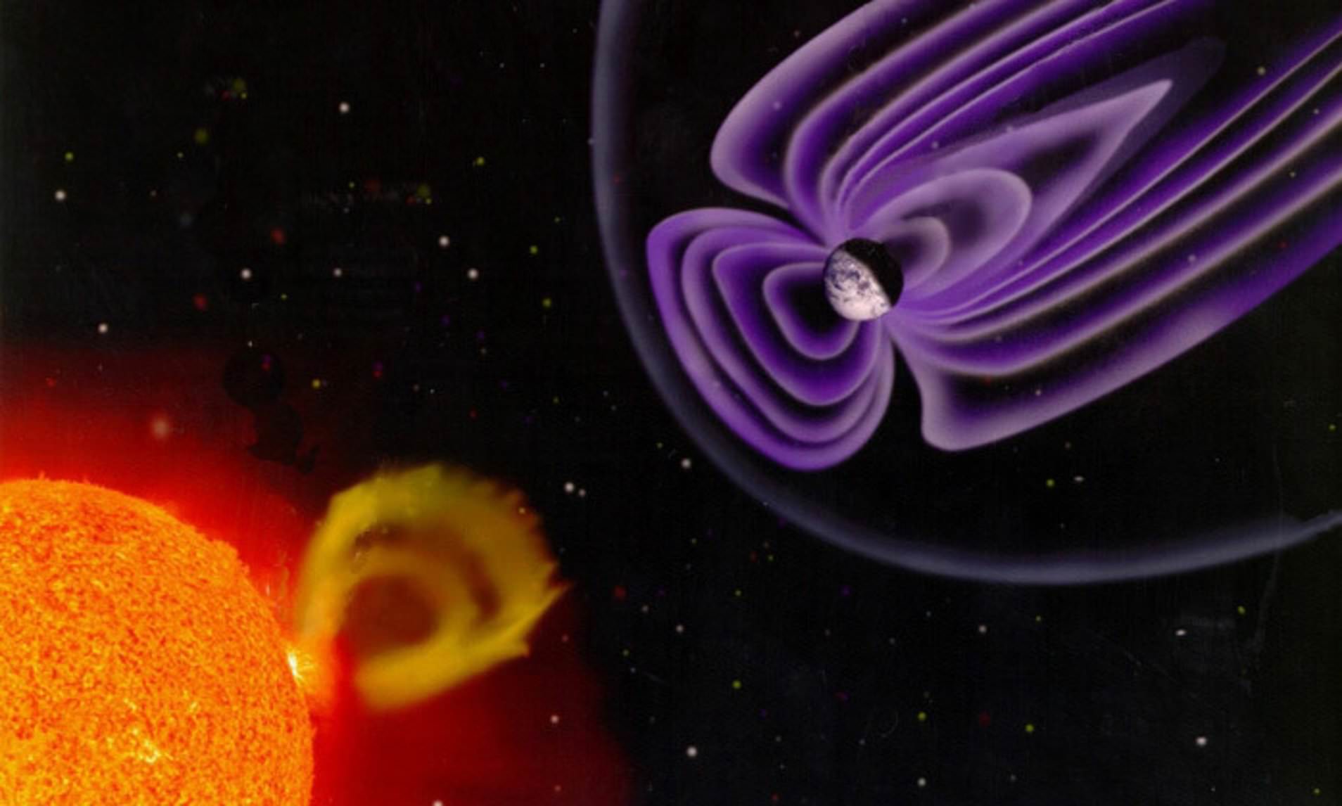
Figure 1: CME Striking the Earth’s Geomagnetic Field
Geomagnetic Storms
CME’s and coronal holes throw clouds of charged particles into space at very high velocities. These clouds of charged particles leave the sun with its magnetic field and can interact with the earth’s magnetic field. Figure 1 shows a CME striking the earth’s geomagnetic field.
The CME is composed of Protons, Electrons, Alpha particles and some heavier particles, and carry the sun’s magnetic field. When this material impacts the earth’s geomagnetic field, it can cause turbulence and disruptions in the ionosphere creating an Ionospheric Storm. The travel time for this material is between 1 and 3 days and its effects include depression of the Critical Frequency and increased absorption. Under severe conditions, the increased geomagnetic activity can disrupt power grids and damage satellites.
The sun constantly emits material that include Electrons, Protons and Alpha particles, and this constitutes the IMF (Interplanetary Magnetic Field). This material has a velocity that averages 360 km/sec, is highly ionized and carries with it the magnetic field of sun. Figure 2 shows the IMF heliospheric current sheet or “ballerina skirt” pattern. The earth is located within the “skirt” area and therefore is periodically subjected to both north and south polarity magnetic field solar wind. When the earth crosses a current sheet polarity boundary, a minor geomagnetic disturbance, G1 storm, maybe generated. The velocity of the solar wind varies with time and can generate a CIR, Co-rotating Interaction Region, as faster solar wind catches up with the slower wind. If the CIR generates a shock front, it can generate minor geomagnetic storm activity when this shock front hits the earth.
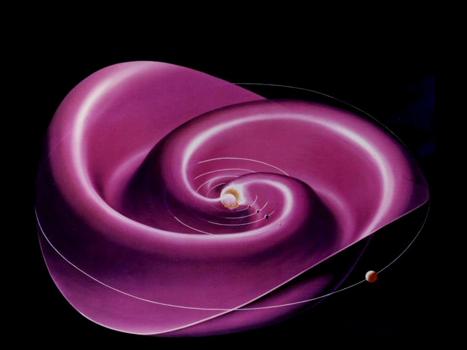
Figure 2: Heliospheric Current Sheet from Sun
A Coronal Hole, seen in Figure 3, is a magnetic weakness or hole in the sun’s Corona, that allows higher speed solar material to mix with the IMF. The combined solar wind velocity can exceed 750 km/sec and cause Geomagnetic Storms similar to a moderate CME. The geomagnetic effects will be more severe when the solar wind has a southern or negative Bz component to the IMF.
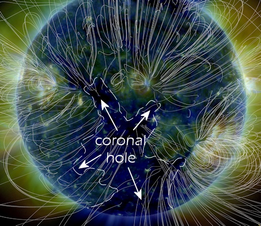
Figure 3: Solar Coronal Hole
Two measurement indices (K and A) are used to express the variation of the earth’s magnetic field from a base-line quiet condition. Quiet solar wind conditions are on the order of 300 to 400 km/sec and originate from the sun’s equatorial or streamer belt. Disruptive solar wind conditions are on the order of 750 km/sec and originate from either Coronal Holes or CME’s. The typical density of these winds is about 1 proton/cm3 but can range up to as high as 50 proton/cm3. The K-index is a three hour measurement of the logarithmic variation of the magnetic field compared to that of a “quiet” day.
An example of a CME impact on the earth can be seen in the next three figures. Figure 4 shows the CME leaving the sun. This is an image from STEREO Ahead positioned about 90º ahead of the earth in the earth orbital plane. This CME took about 3 days to travel from the sun to the earth. The magnetometer on the GOES satellite detected the magnetic effect on the earth geomagnetic field as seen in Figure 5. The ground mounted magnetometers around the earth also responded with a dramatic increase in Kp as seen in Figure 6.
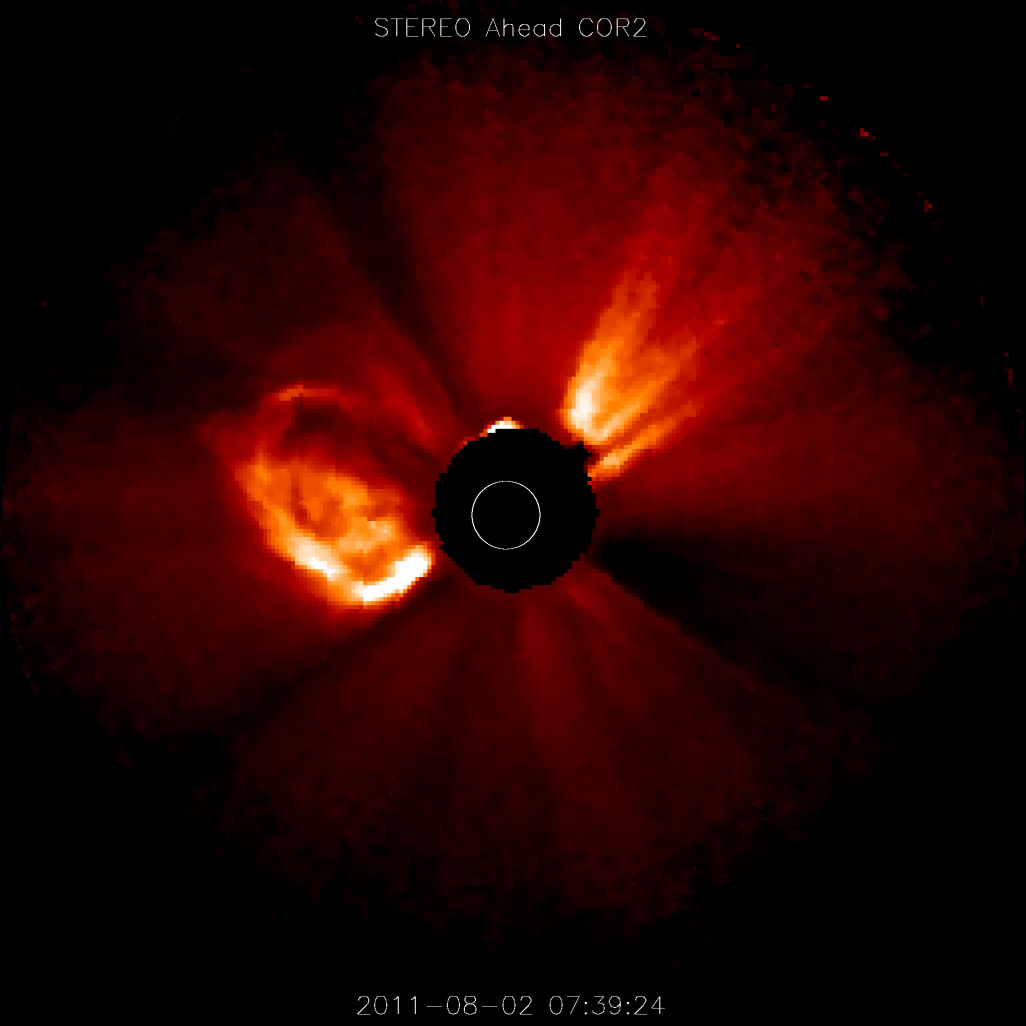
Figure 4: STEREO Ahead Shows CME of 2 AUG 2011 Leaving Sun
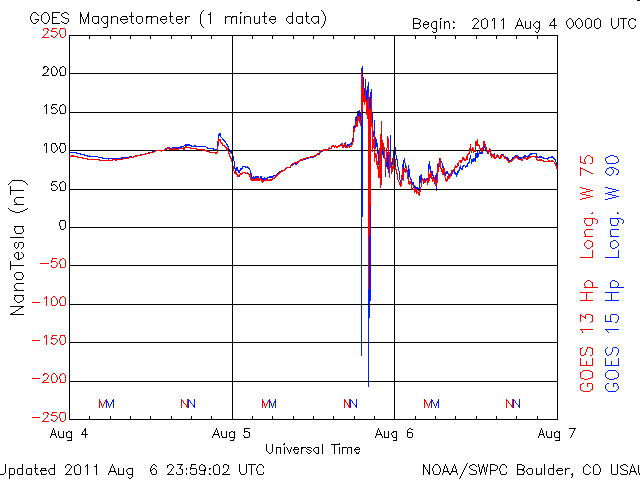
Figure 5: GOES Magnetometer Shows Arrival of CME of 4 AUG 2011
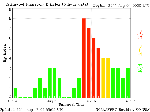
Figure 6: Kp Bar Graph of CME of 4 AUG 2011
Solar Radiation Storms
Solar disturbances may eject vast quantities of high-energy protons. These protons typically take about four hours to reach the earth and will be directed by the earth’s magnetic field into the polar regions. This will result in a Polar Cap Absorption event, a dramatic increase in D-absorption only in the polar regions. Unless very severe, only ionospheric propagation that passes through the polar regions will be effected. Figure 7 shows Proton Flux from GOES 13 satellite. The resulting Polar D-absorption can be seen in Figure 8. Note that there is no absorption for mid-latitudes, so NVIS (Near Vertical Incident Skywave) and longer range skip propagation across the US would not be affected.
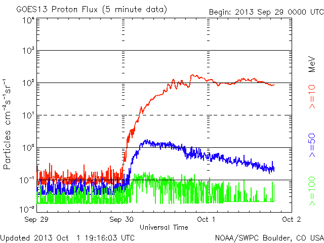
Figure 7: GOES 13 Proton Flux
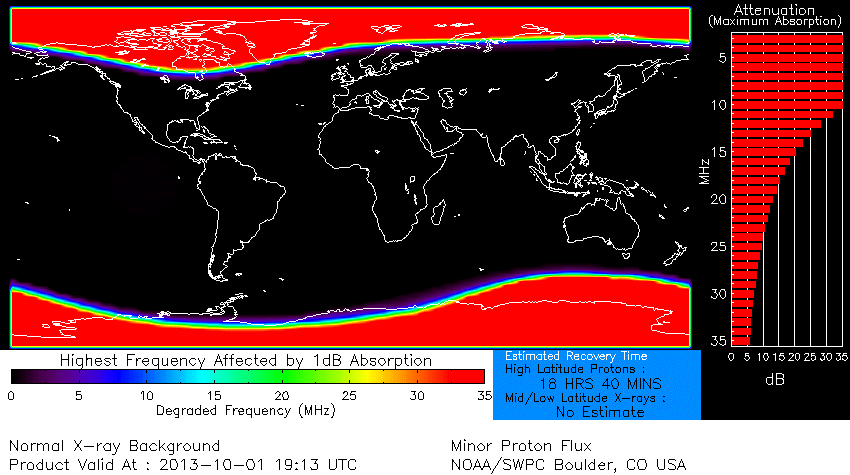
Figure 8: D-Layer Absorption Graph for Proton Event
Radio Blackouts
X-ray radiation from the sun is scaled logarithmically from A, B, C then to M and X in increasing intensity. A large M or X class solar flare generates high levels of x-rays that increase the D-layer absorption, producing a radio blackout called a Sudden Ionospheric Disturbance (SID). The increase in D-layer absorption is due to ionization of Nitrogen and Oxygen molecules in the layer by x-rays from the solar flare. A picture of a large Solar Flare can be seen in Figure 9.
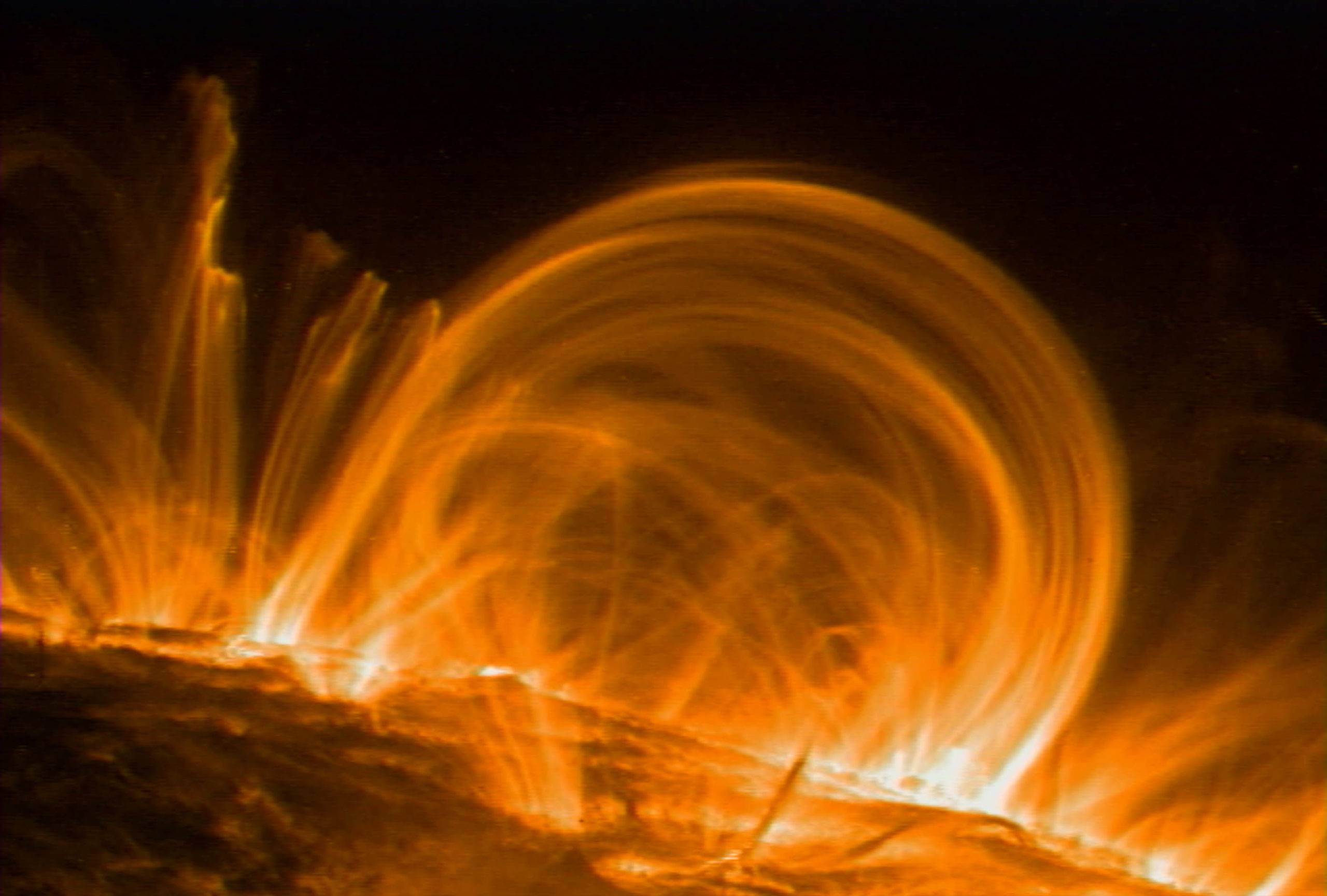
Figure 9: Solar Flare
Since x-rays are electromagnetic radiation, they travel at the speed of light, so there is no warning unlike CME and Coronal Hole disturbances. A SID is a daylight effect and the D-layer will quickly return to normal as soon the flare ends or the earth rotates away from the sun. The GOES x-ray flux for a large X7.4 flare can be seen in Figure 10. The red, 1.0 – 8.0 A, is the x-ray wavelength that penetrates to the D-Layer.
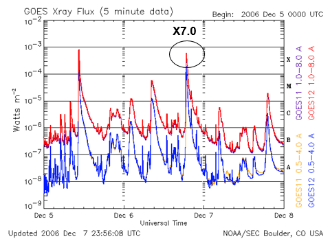
Figure 10: GOES 12 X-Ray Flux For X7.4 flare
Figure 11 shows the resulting D-layer absorption geographically (center plot). The level of D-layer absorption versus frequency can be seen in the bar graph on the right side of Figure 11. NVIS and long-range skip communications would be impossible for this event until the x-ray flux dropped below about C1. The D-layer absorption is a function of 1/f 2 (frequency squared), so operating at a higher frequency may be possible. Note that there is only about 5 dB of attenuation at 20 MHz, so contacting an Amateur station on either coast might allow message traffic to be relayed back into Central Texas. Fortunately, the high density of the gas in the lower-altitude D-layer allows rapid recombination (elimination of absorbing ions), so, as soon as the x-ray flux from the sun ends, the absorption disappears.
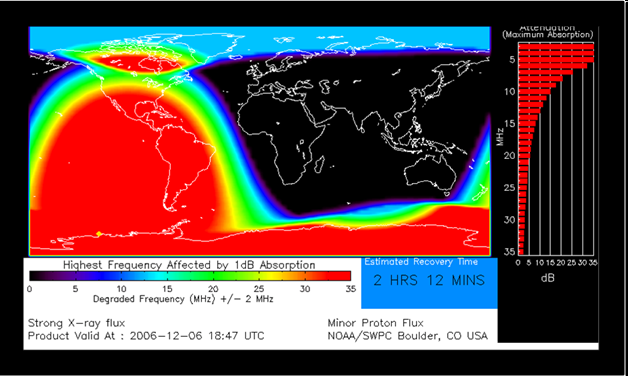
Figure 11: Shows D-layer Absorption for X7.4 Solar Flare Event
With careful attention to solar conditions Amateurs can be prepared to understand and compensate for detrimental effects. This compensation can take the form of adjusting operating frequencies and possibly the use of more robust digital modes. Adjusting our operating parameters to compensate for Space Weather is no different than an ancient sailor adjusting his sails and heading to compensate for varying terrestrial weather conditions.